Polynomial hierarchy
In computational complexity theory, the polynomial hierarchy is a hierarchy of complexity classes that generalize the classes P, NP and co-NP to oracle machines. It is a resource-bounded counterpart to the arithmetical hierarchy and analytical hierarchy from mathematical logic.
Contents |
Definitions
There are multiple equivalent definitions of the classes of the polynomial hierarchy.
- For the oracle definition of the polynomial hierarchy, define
 , and
, and  is the class of problems solvable in polynomial time with an oracle for some NP-complete problem.
 - For the existential/universal definition of the polynomial hierarchy, let
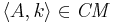
 be a language (i.e. a decision problem, a subset of {0,1}*), let
  be a polynomial, and define
 is some standard encoding of the pair of binary strings x and w as a single binary string. L represents a set of ordered pairs of strings, where the first string x is a member of
  , and the second string w is a "short" (
 ) witness testifying that x is a member of . In other words,
  if and only if there exists a short witness w such that
  . Similarly, define
 and
and  , where Lc is the complement of L. Let
  be a class of languages. Extend these operators to work on whole classes of languages by the definition
 and
and  , where
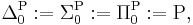
  . The classes NP and co-NP can be defined as
  , and
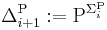
, and 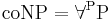 , where P is the class of all feasibly (polynomial-time) decidable languages. The polynomial hierarchy can be defined recursively as
 , and
, and 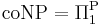 . This definition reflects the close connection between the polynomial hierarchy and the arithmetical hierarchy, where R and RE play roles analogous to P and NP, respectively. The analytic hierarchy is also defined in a similar way to give a hierarchy of subsets of the real numbers.
 - An equivalent definition in terms of alternating Turing machines defines
 (respectively,
  ) as the set of decision problems solvable in polynomial time on an alternating Turing machine with
  alternations starting in an existential (respectively, universal) state.


Relations between classes in the polynomial hierarchy
The definitions imply the relations:

Unlike the arithmetic and analytic hierarchies, whose inclusions are known to be proper, it is an open question whether any of these inclusions are proper, though it is widely believed that they all are. If any  , or if any
  , then the hierarchy collapses to level k: for all
  ,
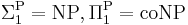
,  . In particular, if P = NP, then the hierarchy collapses completely.
The union of all classes in the polynomial hierarchy is the complexity class PH.
Properties
The polynomial hierarchy is an analogue (at much lower complexity) of the exponential hierarchy and arithmetical hierarchy.
It is known that PH is contained within PSPACE, but it is not known whether the two classes are equal. One useful reformulation of this problem is that PH = PSPACE if and only if second-order logic over finite structures gains no additional power from the addition of a transitive closure operator.
If the polynomial hierarchy has any complete problems, then it has only finitely many distinct levels. Since there are PSPACE-complete problems, we know that if PSPACE = PH, then the polynomial hierarchy must collapse, since a PSPACE-complete problem would be a  -complete problem for some k.
Each class in the polynomial hierarchy contains  -complete problems (problems complete under polynomial-time many-one reductions). Furthermore, each class in the polynomial hierarchy is closed under -reductions: meaning that for a class in the hierarchy and a language
  , if
, if  , then
  as well. These two facts together imply that if
  is a complete problem for
  , then
  , and
, and 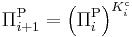 . For instance,
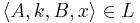
 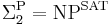 . In other words, if a language is defined based on some oracle in , then we can assume that it is defined based on a complete problem for . Complete problems therefore act as "representatives" of the class for which they are complete.
Sipser–Lautemann theorem states that the class BPP is contained in second level of polynomial hierarchy.
Kannan's theorem states that for any k,  is not contained in SIZE(nk).
Toda's theorem states that the polynomial hierarchy is contained in P#P.
Problems in the polynomial hierarchy
- An example of a natural problem in
 is circuit minimization: given a number k and a circuit A computing a Boolean function f, determine if there is a circuit with at most k gates that computes the same function f. Let be the set of all boolean circuits. The language
is decidable in polynomial time. The language
is the circuit minimization language.
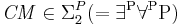 because is decidable in polynomial time and because, given
  ,
,  if and only if there exists a circuit
  such that for all inputs
  ,
,  .
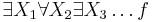
. - A complete problem for is satisfiability for quantified Boolean formulas with k alternations of quantifiers (abbreviated QBFk or QSATk). This is the version of the boolean satisfiability problem for . In this problem, we are given a Boolean formula f with variables partitioned into k sets X1, ..., Xk. We have to determine if it is true that
. The variant in which the first quantifier is "for all", the second is "exists", etc., is complete for .


See also
References
- A. R. Meyer and L. J. Stockmeyer. The Equivalence Problem for Regular Expressions with Squaring Requires Exponential Space. In Proceedings of the 13th IEEE Symposium on Switching and Automata Theory, pp. 125–129, 1972. The paper that introduced the polynomial hierarchy.
- L. J. Stockmeyer. The polynomial-time hierarchy. Theoretical Computer Science, vol.3, pp.1–22, 1976.
- C. Papadimitriou. Computational Complexity. Addison-Wesley, 1994. Chapter 17. Polynomial hierarchy, pp. 409–438.
- Michael R. Garey and David S. Johnson (1979). Computers and Intractability: A Guide to the Theory of NP-Completeness. W.H. Freeman. ISBN 0-7167-1045-5. Section 7.2: The Polynomial Hierarchy, pp.161–167.